Time Series Analysis on Stock Market Data— Explained

TATAMOTORS Data Time Series Analysis

Time series analysis is a specific way of analyzing a sequence of data points collected over an interval of time. In time series analysis, analysts record data points at consistent intervals over a set period of time rather than just recording the data points intermittently or randomly.

Components of Time Series

• Trend: In which there is no fixed interval and any divergence within the given dataset is a continuous timeline. The trend would be Negative or Positive or Null Trend
• Seasonality: In which regular or fixed interval shifts within the dataset in a continuous timeline. Would be bell curve or saw tooth
• Cyclical: In which there is no fixed interval, uncertainty in movement and its pattern
• Irregularity: Unexpected situations/events/scenarios and spikes in a short time span.

https://www.analyticsvidhya.com/blog/2021/10/a-comprehensive-guide-to-time-series-analysis/

Types of Time Series

Stationary: A dataset should follow the below thumb rules without having Trend, Seasonality, Cyclical, and Irregularity components of the time series.

Non- Stationary: If either the mean-variance or covariance is changing with respect to time, the dataset is called non-stationary.

import pandas as pd
import numpy as np
import matplotlib.pyplot as plt
%matplotlib inline
import seaborn as sns
import statsmodels.api as sm
from statsmodels.tsa.seasonal import seasonal_decompose
from statsmodels.tsa.stattools import adfuller
from statsmodels.tsa.stattools import kpss
from statsmodels.graphics.tsaplots import plot_acf, plot_pacf
from statsmodels.tsa.ar_model import AutoReg
from statsmodels.tsa.arima.model import ARIMA
from pandas_datareader import data as pdr
import yfinance as yf
from sklearn.metrics import mean_squared_error

yf.pdr_override()
sns.set_style("whitegrid")

plt.rcParams['figure.figsize'] = (20,6)

df = pdr.get_data_yahoo('TATAMOTORS.ns')
df.tail()

# cuf-off some data
df = df.loc['2022-01-01':,:]
df = df['High']

df.plot(figsize=(20,4))

df = df.reset_index()

df['Date'] = pd.to_datetime(df['Date'])
df = df.set_index(keys='Date'

df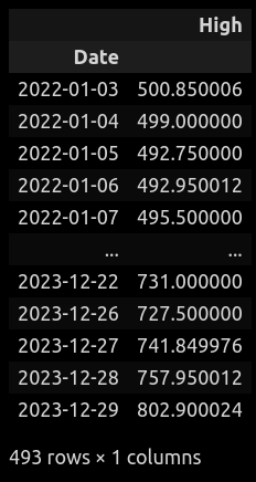

sd = seasonal_decompose(df,model='additive',period=12).plot()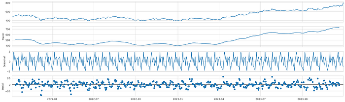

df_log = np.log(df)
df_log.plot()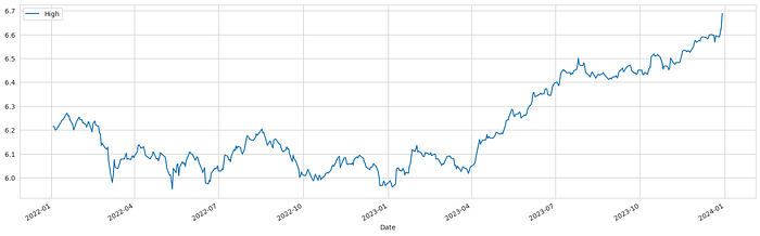

df_log_diff = df_log.diff(periods=3)
df_log_diff.dropna(inplace=True)
df_log_diff.plot()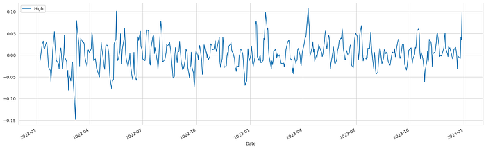

def stationarity_test(df):
    df.dropna(inplace=True)
    rolling_mean = df.rolling(window=12).mean()
    rolling_std = df.rolling(window=12).std()
 
    #plotting all rolling mean and std
    plt.figure(figsize = (13,6))
    plt.xlabel('Years')
    plt.ylabel('No of air pasangers')
    plt.title('Stationary Test: Rolling Mean and Standard Deviation')
    plt.plot(df, color= 'blue', label= 'Original')
    plt.plot(rolling_mean, color= 'green', label= 'Rolling Mean')
    plt.plot(rolling_std, color= 'red', label= 'Rolling Std')    
    plt.legend()
    plt.show()
 
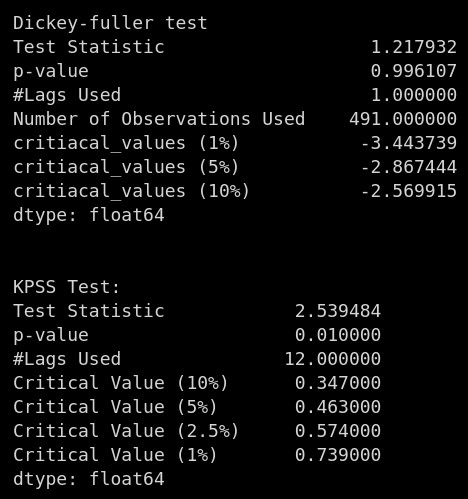
    # Dickey - fuller test for statonarity
    print('Dickey-fuller test')
    df_test = adfuller(df)
    df_op = pd.Series(data = df_test[0:4],index = ['Test Statistic', 'p-value', '#Lags Used', 'Number of Observations Used'])
    for key,value in df_test[4].items():
        df_op['critiacal_values (%s)'%key] = value
    print(df_op)

    print ('\n\nKPSS Test:')
    kpsstest = kpss(df, regression='c', nlags="auto")
    kpss_output = pd.Series(kpsstest[0:3], index=['Test Statistic','p-value','#Lags Used'])
    for key,value in kpsstest[3].items():
        kpss_output['Critical Value (%s)'%key] = value
    print (kpss_output)

stationarity_test(df)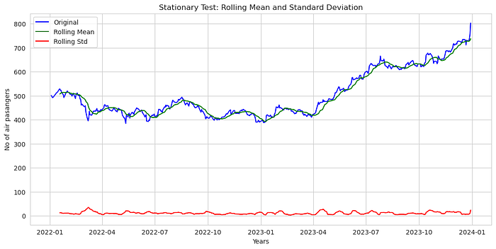

plot_acf(df_log_diff, lags = 25); 
print()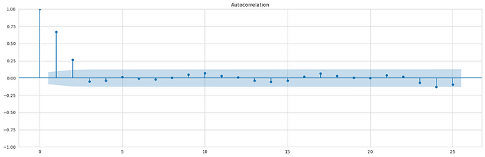

plot_pacf(df_log_diff, lags = 10); 
print()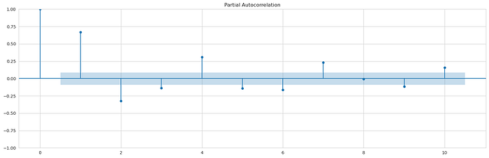

train_size = int(len(df_log_diff) * 0.8)
train, test = df_log_diff[:train_size], df_log_diff[train_size:]

# Function to plot actual vs predicted values
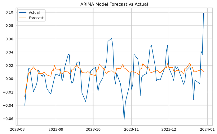
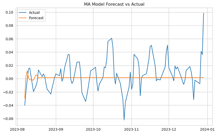
def plot_forecast(test, forecast, model_name):
    plt.figure(figsize=(10, 6))
    plt.plot(test.index, test, label='Actual')
    plt.plot(test.index, forecast, label='Forecast')
    plt.title(f"{model_name} Forecast vs Actual")
    plt.legend()
    plt.show()

ar_model = AutoReg(train.dropna(), lags=10).fit()
ar_forecast = ar_model.predict(start=len(train), end=len(train)+len(test)-1)
print(ar_model.summary())
print('AR Model MSE:', mean_squared_error(test, ar_forecast))
plot_forecast(test, ar_forecast, 'AR Model')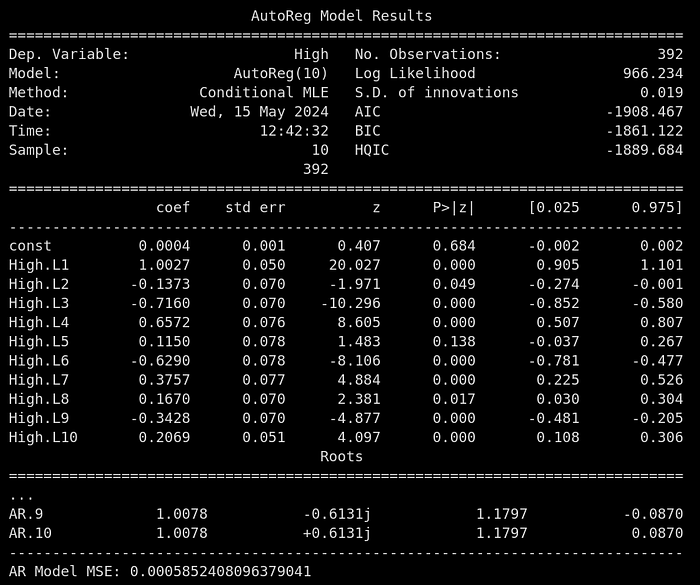

ma_model = ARIMA(train.dropna(), order=(0,0,10)).fit()
ma_forecast = ma_model.predict(start=len(train), end=len(train)+len(test)-1)
print(ma_model.summary())
print('MA Model MSE:', mean_squared_error(test, ma_forecast))
plot_forecast(test, ma_forecast, 'MA Model')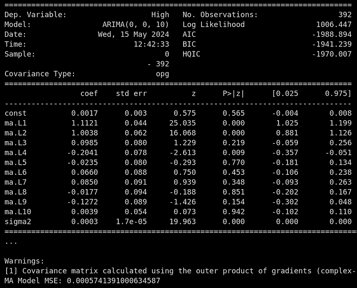

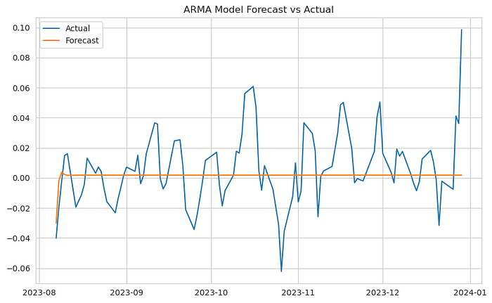
arma_model = ARIMA(train.dropna(), order=(2,0,2)).fit()
arma_forecast = arma_model.predict(start=len(train), end=len(train)+len(test)-1)
print(arma_model.summary())
print('ARMA Model MSE:', mean_squared_error(test, arma_forecast))
plot_forecast(test, arma_forecast, 'ARMA Model')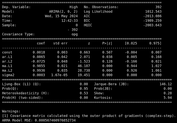

import itertools
p=d=q=range(0,5)
pdq = list(itertools.product(p,d,q))
pdq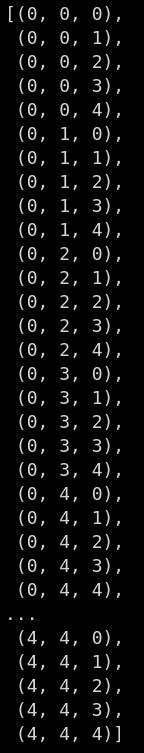

import warnings
warnings.filterwarnings('ignore')
lst = []
train_original = df_log_diff[:train_size]
test_original = df_log_diff[train_size:]
for param in pdq:
    try:
        model_arima = ARIMA(train_original,order=param,seasonal_order=(1,1,1,12))
        model_arima_fit = model_arima.fit()
        arima_forecast = model_arima_fit.predict(start=len(train_original), end=len(train_original)+len(test_original)-1, typ='levels')
        mse = mean_squared_error(test_original, arima_forecast)
        print('ARIMA Model MSE(',param,'):', mse)
        lst.append(mse)

    except:
        continue
# executing for all combinations

train_original = df_log_diff[:train_size]
test_original = df_log_diff[train_size:]
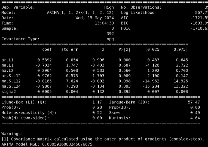
arima_model = ARIMA(train_original, order=(1,1,2),seasonal_order=(1,1,2,12)).fit()
arima_forecast = arima_model.predict(start=len(train_original), end=len(train_original)+len(test_original)-1, typ='levels')
print(arima_model.summary())
print('ARIMA Model MSE:', mean_squared_error(test_original, arima_forecast))
plot_forecast(test_original, arima_forecast, 'ARIMA Model')