A deep dive into Neural Networks, RNN and LSTM
Neural Networks — An Art to Mimic Human Brain
A neural network is a computational model inspired by the way biological neural networks in the human brain process information. These models are a subset of machine learning and are pivotal in the field of artificial intelligence. Neural networks are designed to recognize patterns, make decisions, and predict outcomes based on the data they are trained on.
Key Components of a Neural Network
Neurons (Nodes): A single perceptron receives a set of n-input values from the previous layer. It calculates a weighted average of the values of the vector input, based on a weight vector w and adds bias to the results. The result of this calculation is passed through a non-linear activation function, which forms the output of the unit. The following figure gives a comprehensive idea regarding the summation of n-inputs, post multiplication with the corresponding weights. Prior to taking the output ŷ, the weighted sum is passed through an activation function. In some cases, a bias is added along with the weighted sum, before the activation phase.

Layers:
- Input Layer: The layer that receives the initial data.
- Hidden Layers: Layers between the input and output layers where computations and transformations occur. There can be multiple hidden layers in a deep neural network.
- Output Layer: The final layer that produces the output of the network.

Weights and Biases: Weights determine the importance of each input, while biases help the model make more accurate predictions by shifting the activation function.
Activation Function: A function that determines whether a neuron should be activated or not, adding non-linearity to the model. Common activation functions include ReLU (Rectified Linear Unit), Sigmoid, and Tanh.

Types of Neural Networks
- Feedforward Neural Networks (FNNs): The simplest type, where connections between the nodes do not form cycles. Information moves in one direction — from input to output.
- Convolutional Neural Networks (CNNs): Primarily used for image and video recognition, CNNs utilize convolutional layers to automatically and adaptively learn spatial hierarchies of features.
- Recurrent Neural Networks (RNNs): Suitable for sequential data like time series or natural language, RNNs have connections that form cycles, allowing information to persist.
- Long Short-Term Memory Networks (LSTMs): A type of RNN designed to remember long-term dependencies, which is crucial for tasks like language modeling and time-series prediction.
- Generative Adversarial Networks (GANs): Consist of two networks, a generator and a discriminator, that compete against each other. GANs are used for generating new, synthetic data that resembles the training data.
Learning Algorithm
The learning algorithm consists of two parts — backpropagation and optimization.
Backpropagation: Backpropagation, short for backward propagation of errors, refers to the algorithm for computing the gradient of the loss function with respect to the weights. However, the term is often used to refer to the entire learning algorithm. The backpropagation carried out in a perceptron is explained in the following two steps.
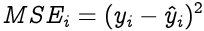
Step 1: To know an estimation of how far are we from our desired solution a loss function is used. Generally, mean squared error is chosen as the loss function for regression problems and cross entropy for classification problems. Let’s take a regression problem and its loss function be mean squared error, which squares the difference between actual (yᵢ) and predicted value ( ŷᵢ ).
Loss function is calculated for the entire training dataset and their average is called the Cost function C.

Step 2: In order to find the best weights and bias for our Perceptron, we need to know how the cost function changes in relation to weights and bias. This is done with the help of the gradients (rate of change) — how one quantity changes in relation to another quantity. In our case, we need to find the gradient of the cost function with respect to the weights and bias.
Let’s calculate the gradient of cost function C with respect to the weight wᵢ using partial derivation. Since the cost function is not directly related to the weight wᵢ, let’s use the chain rule.

Now we need to find the following three gradients

Let’s start with the gradient of the cost function © with respect to the predicted value ( ŷ )

Let y = [y₁ , y₂ , … yₙ] and ŷ =[ ŷ₁ , ŷ₂ , … ŷₙ] be the row vectors of actual and predicted values. Hence the above equation is simplified as

Now let’s find the gradient of the predicted value with respect to the z. This will be a bit lengthy.

The gradient of z with respect to the weight wᵢ is
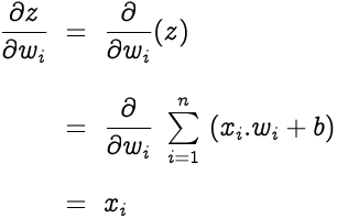
Therefore we get,

Optimization: Optimization is the selection of the best element from some set of available alternatives, which in our case, is the selection of best weights and bias of the perceptron. Let’s choose gradient descent as our optimization algorithm, which changes the weights and bias, proportional to the negative of the gradient of the cost function with respect to the corresponding weight or bias. Learning rate (α) is a hyperparameter which is used to control how much the weights and bias are changed.
The weights and bias are updated as follows and the backpropagation and gradient descent is repeated until convergence.

Recurrent Neural Networks
A Recurrent Neural Network (RNN) is a type of artificial neural network designed to process sequential data. Unlike traditional feedforward neural networks that process data in a one-way flow from input to output, RNNs have loops that allow information to persist and be passed from one step to the next in a sequence. This loop-like structure enables RNNs to exhibit temporal dynamics and capture dependencies across time steps, making it a good fit for sequential data.
The key feature of an RNN is its hidden state, which serves as a memory mechanism that stores information about the past inputs seen in the sequence. At each time step, the RNN takes the current input along with the previous hidden state and computes a new hidden state and output. This recurrent process allows the network to consider the current input in the context of all the previous inputs it has seen so far.
Different architectures and structures
An RNN has a different architecture than a traditional FFNN. Below is an image showing the difference in the architecture of a RNN and a FFNN. Notice the feedback loop in the RNN. On the left side, there’s a representation of a compact, rolled-up RNN. This condensed form hints at the RNN’s cyclic structure, with connections looping back through time steps. On the right side, the RNN is “unrolled”, revealing a series of connected copies of the network, each corresponding to a distinct time step. X0 is in the example above is the stock price on day 0, X1 the price of day 1, etc.

Types of RNN
So we have established that Recurrent neural networks, also known as RNNs, are a class of neural networks that allow previous outputs to be used as inputs while having hidden states. RNN models are mostly used in the fields of natural language processing and speech recognition. Lets look at its types:
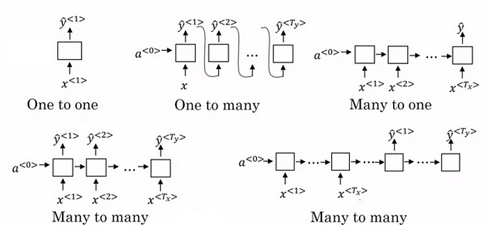
- One to one
- One to many
- Many to one
- Many to many

One to One RNN
One to One RNN (Tx=Ty=1) is the most basic and traditional type of Neural network giving a single output for a single input, as can be seen in the above image.It is also known as Vanilla Neural Network. It is used to solve regular machine learning problems.
One to Many
One to Many (Tx=1,Ty>1) is a kind of RNN architecture is applied in situations that give multiple output for a single input. A basic example of its application would be Music generation. In Music generation models, RNN models are used to generate a music piece(multiple output) from a single musical note(single input).
Many to One
Many-to-one RNN architecture (Tx>1,Ty=1) is usually seen for sentiment analysis model as a common example. As the name suggests, this kind of model is used when multiple inputs are required to give a single output.
Take for example The Twitter sentiment analysis model. In that model, a text input (words as multiple inputs) gives its fixed sentiment (single output). Another example could be movie ratings model that takes review texts as input to provide a rating to a movie that may range from 1 to 5.
Many-to-Many
As is pretty evident, Many-to-Many RNN (Tx>1,Ty>1) Architecture takes multiple input and gives multiple output, but Many-to-Many models can be two kinds as represented above:
1.Tx=Ty:
This refers to the case when input and output layers have the same size. This can be also understood as every input having a output, and a common application can be found in Named entity Recognition.
2.Tx!=Ty:
Many-to-Many architecture can also be represented in models where input and output layers are of different size, and the most common application of this kind of RNN architecture is seen in Machine Translation. For example, “I Love you”, the 3 magical words of the English language translates to only 2 in Spanish, “te amo”. Thus, machine translation models are capable of returning words more or less than the input string because of a non-equal Many-to-Many RNN architecture works in the background.
Limitations and Variants of RNNs
RNNs are great because of their memory in their hidden state, and they don’t take too much RAM to run. There are however some limitations to this. RNNs suffer from vanishing and exploding gradient problems, which make it challenging for them to capture long-range dependencies in sequences.
The vanishing gradient problem refers to a phenomenon in training RNNs, where the gradients used for updating the model’s parameters during backpropagation, diminish exponentially as they are propagated backwards through time or layers. This causes the early layers of the network to receive very small gradient updates, leading to slow or stalled learning, as these layers struggle to effectively adjust their weights and learn meaningful representations from the input data. As a result, the network may have difficulty capturing long-term dependencies and patterns in sequential data.
This can be solved using following methods:
- Weight Initialization
- Choosing the right Activation Function
- LSTM (Long Short-Term Memory) Best way to solve the vanishing gradient issue is the use of LSTM (Long Short-Term Memory).
On the other hand, the problem of exploding gradients envisions this process in reverse, where updated weights become excessively large, rendering the entire network unstable. This situation can lead to numerical overflow and make the network’s training process difficult to control. Both vanishing and exploding gradient problems pose challenges to training deep networks, particularly those handling sequential data like RNNs.
This can be solved using following methods:
- Identity Initialization
- Truncated Back-propagation
- Gradient Clipping
You can see in the example below, where an RNN has to predict the next word. The longer the sentence is, the less influence the first word has on the prediction of the last one.

Additionally, RNNs struggle to retain memory of important information over extended sequences, limiting their ability to effectively process and generate complex patterns.
LSTM
A Long-Short-Term-Memory NN (LSMT) solves these limitations that the RNN is facing. LSTM is a specialised type of RNN architecture that addresses the vanishing and exploding gradient problems associated with traditional RNNs. LSTM is designed to capture and retain long-range dependencies in sequences by introducing mechanisms that control the flow of information through the network, allowing for more effective learning and representation of sequential patterns.
LSTM solves the gradient issue through its unique design, which incorporates three main components: the cell state, hidden state, and gating mechanisms.

Let’s understand these components, one by one.

1. Cell State (Memory cell)
It is the first component of LSTM which runs through the entire LSTM unit. It kind of can be thought of as a conveyer belt.

This cell state is responsible for remembering and forgetting. This is based on the context of the input. This means that some of the previous information should be remembered while some of them should be forgotten and some of the new information should be added to the memory. The first operation (X) is the pointwise operation which is nothing but multiplying the cell state by an array of [-1, 0, 1]. The information multiplied by 0 will be forgotten by the LSTM. Another operation is (+) which is responsible to add some new information to the state.
2. Forget Gate
The forget LSTM gate, as the name suggests, decides what information should be forgotten. A sigmoid layer is used to make this decision. This sigmoid layer is called the “forget gate layer”.

It does a dot product of h(t-1) and x(t) and with the help of the sigmoid layer, outputs a number between 0 and 1 for each number in the cell state C(t-1). If the output is a ‘1’, it means we will keep it. A ‘0’ means to forget it completely.
3. Input gate
The input gate gives new information to the LSTM and decides if that new information is going to be stored in the cell state.

This has 3 parts-
- A sigmoid layer decides the values to be updated. This layer is called the “input gate layer”
- A tanh activation function layer creates a vector of new candidate values, Č(t), that could be added to the state.
- Then we combine these 2 outputs, i(t) * Č(t), and update the cell state.
The new cell state C(t) is obtained by adding the output from forget and input gates.

4. Output gate
The output of the LSTM unit depends on the new cell state.

First, a sigmoid layer decides what parts of the cell state we’re going to output. Then, a tanh layer is used on the cell state to squash the values between -1 and 1, which is finally multiplied by the sigmoid gate output.

